Finite element method
The finite element method (FEM) is a fundamental numerical technique for solving complex differential equations that arise in engineering and scientific modelling. It works by dividing a large system into smaller, simpler parts called finite elements, which are then solved and reassembled to approximate a solution for the entire problem. In Canada, FEM and its practical application, finite element analysis (FEA), are critical tools across industries, from designing safer automobiles and more efficient aircraft to modelling geological processes and advancing biomedical engineering. Its development, spanning from the 1940s to the present, represents a key part of computational science, enabling the simulation and optimization of physical systems before physical prototypes are ever built.
Fundamental Principles and Process
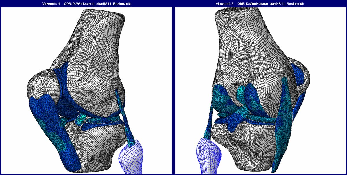
The core principle of the finite element method is the subdivision, or discretization, of a complex, continuous domain into a finite number of smaller, interconnected subdomains known as finite elements. This spatial discretization is implemented by constructing a mesh over the object or region of interest, which consists of a finite set of points called nodes. The behaviour within each simple element is described by relatively straightforward equations, which are derived to approximate the more complex governing equations of the overall physical system. These element equations are then systematically assembled, respecting the connectivity of the mesh, into a much larger global system of algebraic equations or ordinary differential equations that model the entire problem. The process of studying a phenomenon using FEM is universally referred to as finite element analysis (FEA).
The subdivision approach offers several significant advantages for solving real-world engineering problems. It allows for the accurate digital representation of geometries that are highly complex and irregular, which would be intractable with purely analytical mathematical methods. The method readily accommodates dissimilar material properties within a single model, such as a composite aircraft wing made of carbon fibre and metal alloys. This localized modelling also facilitates the easy representation of the total solution across the entire domain while effectively capturing critical local effects, like stress concentrations around a bolt hole or heat flux at a specific boundary. The standard workflow of FEA involves a sequence of well-defined steps, beginning with the creation of a geometric model of the physical system.
The analyst then defines the material properties, applies loads and boundary conditions, and generates a suitable mesh over the geometry. The FEM software, coded with specific algorithms, formulates the element equations based on the chosen physics, such as structural mechanics or fluid dynamics, and assembles the global system. This large system is then solved using numerical linear algebra techniques to compute the primary unknowns, like displacement or temperature, at every node in the mesh. The final stage is post-processing, where the raw solution data is interpreted into useful engineering results like stress contours, deformation animations, or heat flow diagrams to inform design decisions. This entire process replaces multiple cycles of building and testing physical prototypes, saving considerable time and resources.
Historical Development and Key Figures
While a single invention date is difficult to pinpoint, its conceptual foundations were laid in the early 1940s through the independent work of Alexander Hrennikoff and Richard Courant. Hrennikoff employed a lattice analogy to discretize domains, while Courant proposed dividing a domain into finite triangular sub-regions to solve partial differential equations related to the torsion of a cylinder. Courant's work was evolutionary, building upon earlier variational methods developed by Lord Rayleigh, Walther Ritz, and Boris Galerkin. The method was also independently developed in other parts of the world.
In the Soviet Union, the practical application of FEM is often associated with the work of Leonard Oganesyan. In China, mathematician Feng Kang developed similar concepts in the late 1950s and early 1960s based on computations for dam construction, referring to it as the finite difference method based on variation principles. Another significant early pioneer was Ioannis Argyris. Despite their different approaches, all these pioneers shared the essential characteristic of discretizing a continuous domain into a set of discrete sub-domains, or elements. The widespread adoption and maturation of FEM occurred during the 1960s and 1970s, driven by several key research groups and the advent of digital computers.
Critical developments came from J. H. Argyris and his team at the University of Stuttgart, R. W. Clough at the University of California Berkeley, and O. C. Zienkiewicz along with colleagues like Ernest Hinton and Bruce Irons at Swansea University. Other important contributors included Philippe G. Ciarlet at the University of Paris 6 and Richard Gallagher at Cornell University. This period also saw the creation of influential, often open-source, FEM software that propelled the method into industry. NASA sponsored the development of NASTRAN, UC Berkeley released SAP IV and later OpenSees, and the Norwegian ship classification society Det Norske Veritas developed Sesam in 1969 for ship analysis. A rigorous mathematical foundation for the method was solidified in 1973 with a seminal publication by Gilbert Strang and George Fix, which provided a clear mathematical basis for the techniques being used.
Technical Framework and Discretization Strategies
A complete finite element method is characterized by four interconnected components: a variational formulation, a discretization strategy, one or more solution algorithms, and post-processing procedures. The variational formulation, such as the widely used Galerkin method or the discontinuous Galerkin method, transforms the original strong form of the differential equation into an equivalent weak or variational form. This step often involves integration by parts and reduces the continuity requirements on the approximate solution, making it suitable for a wider range of problems. The weak form serves as the starting point for the numerical discretization that follows. The discretization strategy is a clearly defined set of procedures that govern how the physical domain is broken down and how the solution is approximated within each element.
This strategy encompasses the creation of the finite element mesh, the definition of basis functions on reference elements, and the mapping of these reference elements onto the actual elements in the mesh. Over time, several distinct discretization strategies have been developed, each with its own advantages and target applications. The primary strategies include the h-version, the p-version, the hp-version, the extended finite element method (x-FEM), and isogeometric analysis. The choice of discretization strategy aims to achieve nearly optimal performance for the broadest set of mathematical models within a particular class. Following discretization, the resulting large, sparse system of equations must be solved using appropriate numerical algorithms.
- The h-version is the most classical approach, where convergence is achieved by refining the mesh (reducing the element size 'h') while keeping the polynomial order of the basis functions fixed.
- The p-version refines the solution by increasing the polynomial order ('p') of the basis functions on a fixed mesh.
- The hp-version combines both techniques, simultaneously refining the mesh and increasing the polynomial order, which can achieve exponential rates of convergence for certain problems.
- The extended finite element method (x-FEM) enriches the standard approximation space with special functions to model internal boundaries, like cracks, without requiring the mesh to conform to them.
- Isogeometric analysis seeks to integrate finite element analysis with computer-aided design by using the same functions for geometric modelling and analysis, typically Non-Uniform Rational B-Splines (NURBS).
Various numerical solution algorithms for finite element methods can be classified into two broad categories, which are direct and iterative solvers. These algorithms are designed to exploit the sparsity of matrices that depend on the choices of variational formulation and discretization strategy. Post processing procedures are designed to extract the data of interest from a finite element solution. To meet the requirements of solution verification, postprocessors need to provide for a posteriori error estimation in terms of the quantities of interest. When the errors of approximation are larger than what is considered acceptable, then the discretization has to be changed. A finite element method is characterized by a variational formulation, a discretization strategy, one or more solution algorithms, and post processing procedures.
Core Mathematical Illustration
The mathematical foundation of FEM is often illustrated through two classic boundary value problems. The first, known as P1, is a one-dimensional problem defined on the interval (0,1) where the second derivative of an unknown function u(x) equals a given function f(x), with boundary conditions u(0)=u(1)=0. While this simple problem can be solved directly via antiderivatives, it serves to demonstrate the FEM process which generalizes to higher dimensions. The second problem, P2, is a two-dimensional Dirichlet problem where the sum of the second partial derivatives of u(x,y) with respect to x and y equals f(x,y) within a domain Ω, with u=0 on the boundary ∂Ω. This problem is representative of many physical scenarios, such as steady-state heat conduction.
The FEM solution for these problems proceeds in two essential steps that mirror the general technical framework. The first step is to convert the original strong-form boundary value problem into its equivalent weak or variational formulation. For P1, this involves multiplying the differential equation by a smooth test function v(x) that satisfies the boundary conditions, integrating over the domain, and using integration by parts to transfer a derivative from the unknown u onto the test function v. This results in a bilinear form φ(u,v) that is equal to a linear functional defined by f and v. The weak form only requires u to have one derivative, whereas the original form required two, thus broadening the space of admissible solutions. The second step is the discretization of this weak form.
The infinite-dimensional function spaces are replaced by finite-dimensional subspaces. For a one-dimensional mesh of the interval (0,1), piecewise linear basis functions, often called hat functions, are defined such that each function is 1 at its associated node and 0 at all other nodes. The unknown solution u(x) is approximated as a linear combination of these basis functions. Substituting this approximation into the weak form and choosing the test functions v to be the same basis functions leads to a finite-dimensional system of linear algebraic equations, known as the Galerkin system. The solution of this system yields the coefficients of the basis functions, which define the approximate FEM solution across the entire domain. This process demonstrates how a continuous differential equation is transformed into a discrete algebraic problem suitable for computer solution.
Applications in Engineering and Science
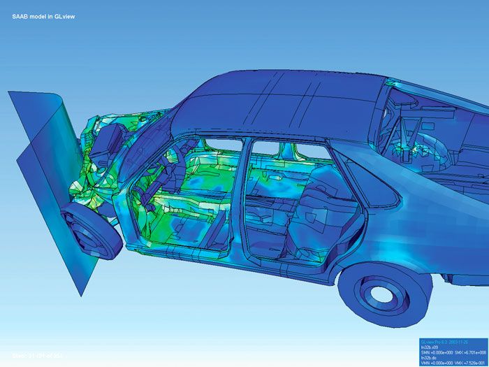
Finite element analysis has become an indispensable computational tool across virtually every field of engineering and applied science due to its versatility in handling complicated domains, changing geometries, and varying material properties. In mechanical and aerospace engineering, FEA is routinely used for structural analysis to predict stresses, strains, and deformations in components ranging from engine brackets to entire aircraft wings under load. It is crucial for performing static, dynamic, and buckling analyses, as well as for simulating complex events like crashworthiness in vehicles, where it allows engineers to optimize safety features and reduce the need for expensive physical crash tests. The ability to increase solution accuracy in critical areas, like the front of a car in a frontal impact simulation, while reducing it in less critical areas, makes FEA both powerful and computationally efficient.
In the field of heat transfer and thermal engineering, FEA solves the heat equation to model conduction, convection, and radiation. Applications include designing heat sinks for electronics, analyzing thermal stresses in engine components, and optimizing building insulation. In fluid dynamics, while computational fluid dynamics (CFD) often uses the finite volume method, FEM is also employed to solve the Navier-Stokes equations for modelling fluid flow around objects, in pipelines, or within chemical processing equipment. Coupled physics problems, such as fluid-structure interaction where aerodynamic forces deform a structure which in turn alters the flow, are also tackled using advanced FEA techniques. The method's reach extends far beyond traditional mechanical fields.
In civil engineering, it is used to analyze the behaviour of dams, bridges, and skyscrapers under seismic loads. In electrical engineering and electromagnetics, FEM solves Maxwell's equations for designing motors, transformers, and antennas. Biomedical engineers use it to model bone mechanics, stent deployments, and soft tissue behaviour. Geoscientists apply FEA to model rock deformation and fault mechanics. The common thread is the need to solve partial differential equations or integral equations over domains that are too geometrically complex or physically nonlinear for analytical solutions, making FEA a universal tool for virtual prototyping and scientific discovery that has transformed modern design and analysis practices.
The Finite Element Software Ecosystem
The practical implementation of the finite element method relies heavily on sophisticated software, creating a vast and mature commercial and academic ecosystem. These software packages integrate all stages of the FEA workflow: pre-processing for geometry creation and meshing, solvers that implement the core FEM algorithms, and post-processors for visualization and results interpretation. The development of such software was instrumental in the method's proliferation from academic research to industrial practice. Early influential programs, many of which were open-source or publicly available, provided a foundation for later commercial developments. Historically significant programs include NASTRAN, originally developed with NASA sponsorship for structural analysis in the aerospace industry.
The University of California Berkeley contributed SAP IV, a widely used structural analysis program, and later OpenSees, an open-source framework for simulating the seismic response of structural and geotechnical systems. In Europe, the SESAM program was developed in 1969 by Det Norske Veritas for the analysis of ship structures. These programs demonstrated the power of FEM and spurred the growth of a commercial software market. Today, the landscape is dominated by comprehensive multiphysics suites that integrate FEA with other simulation tools. These modern platforms offer extensive capabilities for modelling nonlinear materials, complex contact conditions, and multiple coupled physical phenomena, which are essential for solving today's advanced engineering challenges.
| Software | Primary Developer/Company | Notable Features/Application Focus |
|---|---|---|
| ABAQUS | Dassault Systèmes | Advanced nonlinear and multiphysics analysis |
| ANSYS | ANSYS, Inc. | Comprehensive multiphysics suite (structural, fluids, electromagnetics) |
| COMSOL Multiphysics | COMSOL | Equation-based modelling for coupled physics phenomena |
| LS-DYNA | LSTC (Livermore Software Technology Corp.) | Explicit dynamics for crash, impact, and blast simulations |
| MSC Nastran | Hexagon (MSC Software) | Industry-standard for linear and nonlinear structural analysis |
| OpenFOAM | OpenFOAM Foundation | Open-source toolbox primarily for CFD, uses finite volume method |
| OpenSees | Pacific Earthquake Engineering Research Center | Open-source framework for seismic simulation |
The practical application of the finite element method is known as finite element analysis. Finite element analysis includes the use of mesh generation techniques for dividing a complex problem into smaller elements. It also includes the use of software coded with a finite element method algorithm. During the 1960s and 1970s, additional impetus for finite element method development was provided by available open source programs. For example, NASA sponsored the original version of NASTRAN, and the University of California Berkeley made the finite element programs SAP IV and later OpenSees widely available. The method has since been generalized for the numerical modeling of physical systems in a wide variety of engineering disciplines.
Canadian Context and Industry Impact
In Canada, the finite element method is a critical enabling technology for the nation's key industrial and research sectors. The Canadian aerospace industry, a global leader, relies extensively on FEA for the design, analysis, and certification of aircraft and spacecraft components. Companies like Bombardier (now part of Airbus for the A220 program), Pratt & Whitney Canada, and CAE use advanced FEA to simulate structural integrity under flight loads, optimize lightweight materials like composites, and model complex fluid-structure interactions for wings and engine parts. This virtual testing is essential for meeting stringent international safety regulations while reducing development time and cost. The automotive sector in Canada, including manufacturing plants for global manufacturers and domestic suppliers, utilizes FEA for vehicle design and crash simulation.
The method helps engineers design safer vehicle crumple zones, more durable chassis components, and quieter cabins by simulating noise, vibration, and harshness (NVH). In the resource industries, FEA is applied to model the structural behaviour of mining equipment, analyze the integrity of pipelines carrying oil and gas across vast distances, and assess the stability of tailings dams. Civil engineers across the country use FEA to design earthquake-resistant buildings and bridges, particularly important in seismically active regions like British Columbia. Academic and government research in Canada also heavily employs and contributes to FEM development, with universities and national labs conducting advanced research.
Universities with strong engineering programs, such as the University of Toronto, University of British Columbia, McGill University, and University of Waterloo, host research groups that advance FEM theory and applications. Research areas include developing new discretization methods, applying FEA to biomedical problems like bone implant design and cardiovascular flow, and modelling climate-related processes such as permafrost thaw and glacier mechanics. Government laboratories, including those within the National Research Council Canada, use FEA for materials research and to support industrial innovation. This widespread adoption confirms FEM's role as a fundamental tool for Canadian technological competitiveness and scientific advancement across multiple economic and research domains.
Questions about Finite element method
What is the difference between FEM and FEA?
The terms are closely related but have a subtle distinction. The finite element method (FEM) refers to the broad mathematical framework and numerical technique for solving differential equations by discretizing a domain into finite elements. Finite element analysis (FEA) is the practical application of this method to solve specific engineering or scientific problems. In everyday usage, especially in industry, the term FEA is more commonly used to describe the overall process of computer-aided simulation using the finite element method. So, FEM is the theory, and FEA is the practice of implementing that theory to analyze real-world systems.
What are the main advantages of using finite element analysis?
Finite element analysis offers several key advantages over traditional analytical methods and physical prototyping. It can accurately model and analyze systems with extremely complex geometries that are impossible to solve by hand. FEA can easily incorporate different material properties within a single model and simulate complex loading and boundary conditions. It allows engineers to capture local effects, like stress concentrations, with high precision. Perhaps most importantly, FEA enables virtual prototyping, where designs can be tested, optimized, and validated computationally before any physical prototype is built. This dramatically reduces development costs, shortens design cycles, and allows for the exploration of more design alternatives while improving product performance and safety.
What types of problems can FEA solve?
FEA is a versatile tool capable of solving a wide range of physical problems governed by differential equations. The most common applications are in structural mechanics for stress, strain, vibration, and buckling analysis. It is also extensively used for thermal analysis to model heat transfer via conduction, convection, and radiation. In fluid dynamics, FEA can solve problems related to laminar and turbulent flow, though the finite volume method is also popular in this domain. Other major application areas include electromagnetics for designing motors and antennas, acoustics for noise control, and coupled multiphysics problems where phenomena like thermal stress or fluid-structure interaction occur. Essentially, any physical system that can be described mathematically can potentially be analyzed using FEA.
What are the basic steps involved in an FEA?
A typical finite element analysis follows a systematic workflow. The first step is pre-processing, which involves creating or importing a geometric model of the part or system, defining the material properties, applying the appropriate loads and boundary conditions, and generating a finite element mesh over the geometry. The second step is solution, where the FEA software assembles the global system of equations based on the physics being simulated and solves this large numerical system to compute primary unknowns like displacement or temperature at each node. The final step is post-processing, where the engineer interprets the results using colour contour plots, deformation animations, graphs, and reports to evaluate factors of safety, identify failure points, and make informed design decisions. Verification and validation of the model against known results or physical tests are also critical parts of the process.
Who were the key pioneers in developing the finite element method?
The development of FEM was a collaborative, international effort spanning decades. Key early pioneers in the 1940s included Alexander Hrennikoff, who used a lattice analogy, and Richard Courant, who used triangular subdivisions. Ioannis Argyris was another significant early contributor. The method gained major momentum in the 1960s and 1970s through the work of several research groups. J. H. Argyris at the University of Stuttgart, R. W. Clough at UC Berkeley, and O. C. Zienkiewicz at Swansea University were instrumental in advancing and promoting the method. Other important figures included Philippe G. Ciarlet and Richard Gallagher. In 1973, Gilbert Strang and George Fix provided a rigorous mathematical basis for the method. Parallel developments occurred in the USSR with Leonard Oganesyan and in China with Feng Kang.
How is FEA used in the Canadian industry?
FEA is a critical technology across Canada's major industrial sectors. In aerospace, companies like Pratt & Whitney Canada use it to design and certify jet engine components, while others use it for airframe structural analysis. The automotive industry employs FEA for crash simulation, durability testing, and noise reduction in vehicles manufactured in Canada. In the natural resources sector, FEA is critical for analyzing the integrity of pipelines, designing mining equipment, and assessing the safety of dams and tailings ponds. Canadian civil engineering firms rely on FEA to design earthquake-resistant infrastructure, especially in British Columbia. Canadian universities and research institutes are active in advancing FEM methodologies and applying them to fields like biomedical engineering and environmental science, ensuring the country remains at the forefront of computational engineering.
Sources and further reading
- Finite element method (Wikipedia)
- Unveiling the History of the Finite Element Method (consulting.artem.co.in)
- Finite element method in engineering and structural design (amusementlogic.com)
Checked by the Your Space Hamilton desk. Last updated 2026-10-20.